We posted previously on the exceptional movements of Franklin’s Gulls and Cave Swallows that occurred around 13 November 2015. The first post set the stage for how these species appeared so far out of range, and we follow with this post about some rumination about why this event took place. Here, we consider the combined effects of a strong mid-latitude cyclone as the primary factor (how) and anomalously warm temperatures in the typical October and early November distribution of at least one of these species (why). We will focus on Franklin’s Gull, here, and in part three of our story we will focus on Cave Swallow.
Let’s explore a possible connection between strong cyclonic storms and the migration conditions in the typical distribution range of Franklin’s. eBird range maps for the occurrence of Franklin’s Gull are below. First, note that Franklin’s Gull, which is a strongly migratory species with an exceptionally long-distance route to travel between hemispheres, shows the strongest (dark purple = higher percentage of complete checklists reporting the species) signal from the central US.
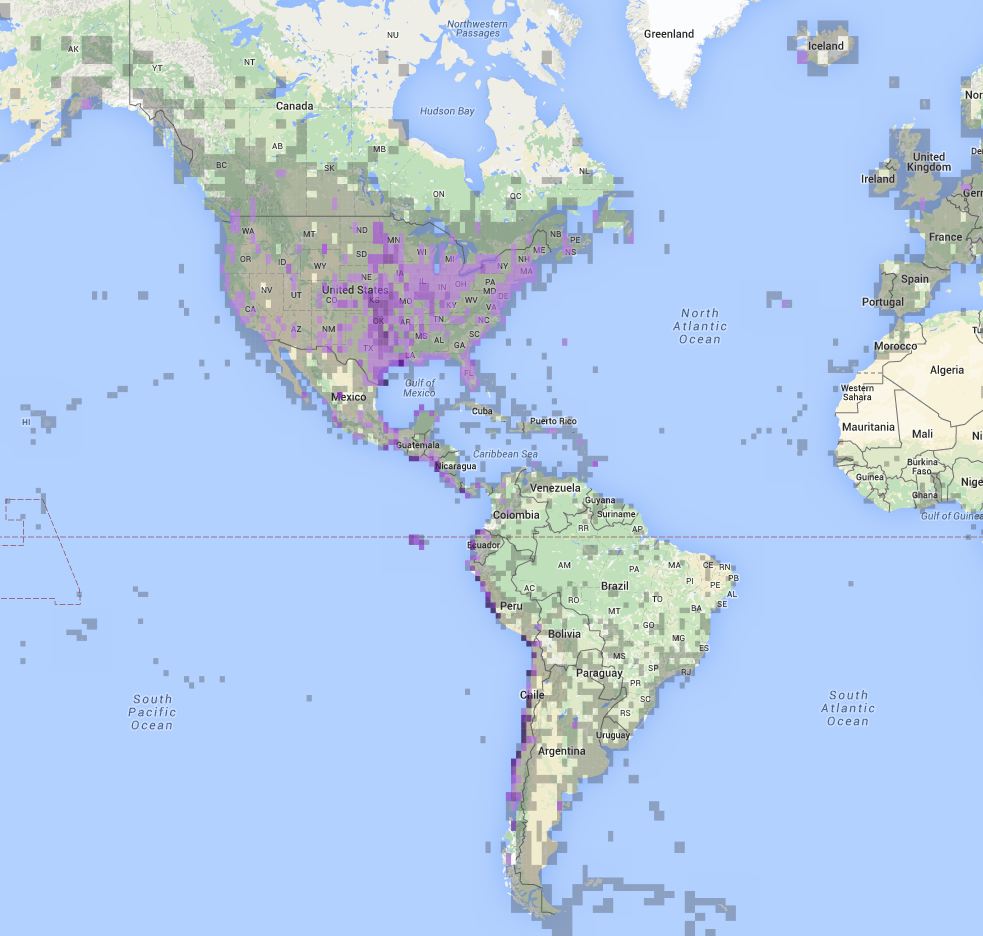
Franklin’s Gull eBird range map, November, 1995-2015.
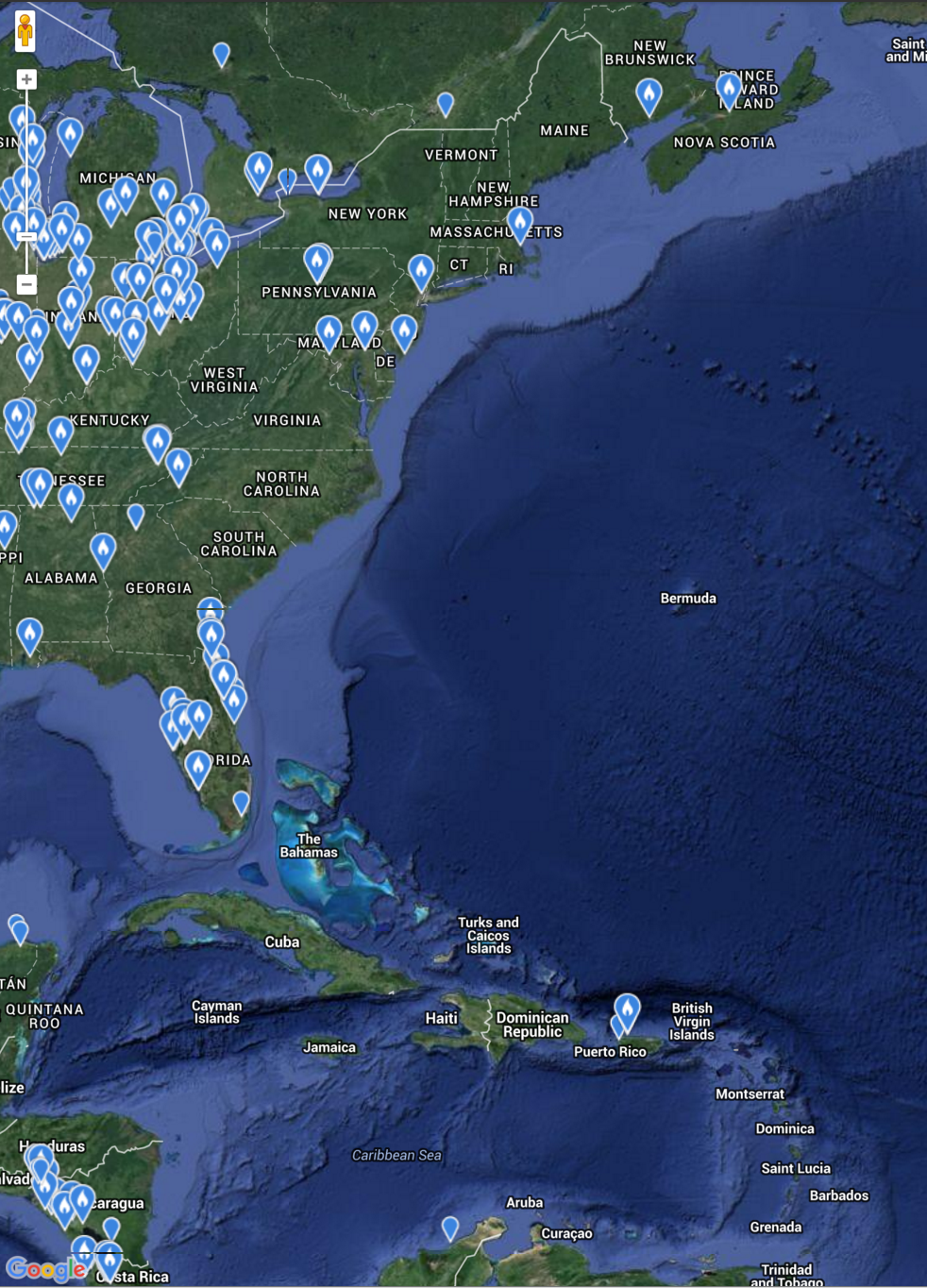
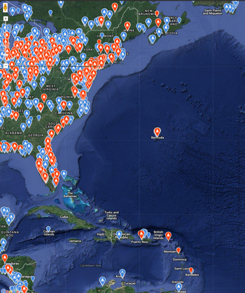
Next, compare the 2014 Franklin’s Gull map (upper; typical of most years, with just a small handful of records on the East Coast (mostly in Florida) with the map from 2015 (lower map; November-December records in red). Not shown on the 2015 map is an Iceland record and a couple recent Caribbean records as the birds from the invasion have worked their way south (most Florida records from 2015 appear to be birds filtering south along the coast). Note the strong Great Lakes and East Coast prevalence in the 2015 invasion. There surely would have been more inland records if observers had mobilized faster on the day of the invasion–13 November–and if the invasion had happened on a weekend instead of a weekday.

Finally, below is the same map but for all time, showing how dominant the 2015 records are. The November 2015 records are the red dots; most of the blue dots are from prior years.
Let’s also see how temperature anomalies in the US relate to this story, both during the month preceding the November 1998 movements and the month and weeks preceding the 2015 movements.
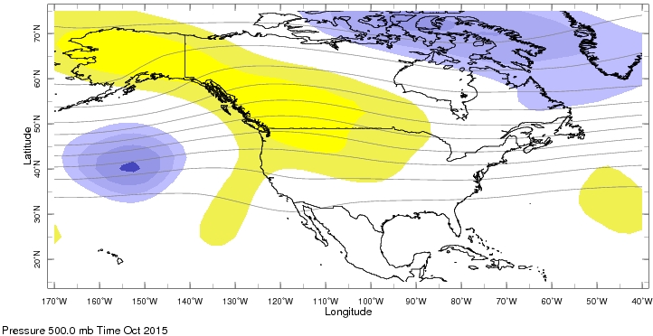
Here is a map of temperature anomalies for October 2015 (see this site for methodologies to generate these data). The yellows and oranges correspond to areas with above normal temperatures, and the blues correspond to areas with below normal temperatures.
Additionally, here is a map of October 1998 temperature anomalies.
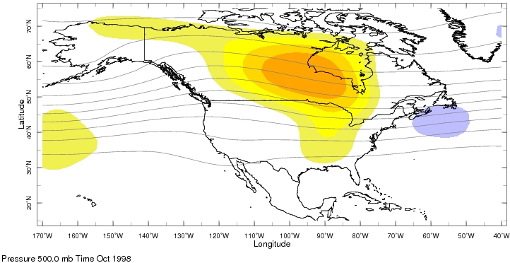
Both of these images highlight a warmer than normal zone in the middle of the country, slightly different in distribution between the years. However, both years have in common anomalies that occurred in the northern Plains and Upper Midwest. These temperature anomalies are important for two reasons: 1) abnormally warm years may create weather pattern that “bottles-up” Franklin’s Gulls in the Upper Midwest; 2) these abnormally warm years are more likely to produce the storm storms witnessed in 1998 and 2015. We would suggest that these two factors in concert are the primary explanations for this year’s movement.
These lobes of warm weather in October of 1998 and 2015 are remarkably similar. During these periods, typical fall migration weather (cool northerly winds after cold fronts) are unusually scarce. Further analyses will look at whether Franklin’s Gulls were in fact unusually common in the Upper Midwest prior to this year’s invasion; if so, this may be an important correlative factor with this year’s massive invasion. Additionally, warmer than average temperatures in the region certainly associate with more intense storms systems – the boundary between a seasonally appropriate cool air mass and a seasonally anomalous warmer than average air mass is dynamic and turbulent, producing an environment where strong storms are likely: there is more heat to fuel the storms and greater differences between cool and warm air masses facilitating the growth of such storms.
A third possible causal relationship should be investigated: did Franklin’s Gulls have an exceptionally good breeding year, leading to a much higher overall population? This article points out the obvious connection: overall population spikes correlate with increased vagrancy. In 2015, this might be suggested by first-winter birds appearing out of range prior to the invasion in Florida, New Brunswick, and Maine. In most areas on the East Coast, first-winter birds predominated, which could suggest a good breeding year (or alternatively, that young birds were more prone to displacement in this storm, either through later lingering in the source areas or relatively higher entrainment in the system). However, a large percentage of birds at Cape May were adults – clearly, a full analysis of the ages involved in the 2015 records is needed (and presently underway).
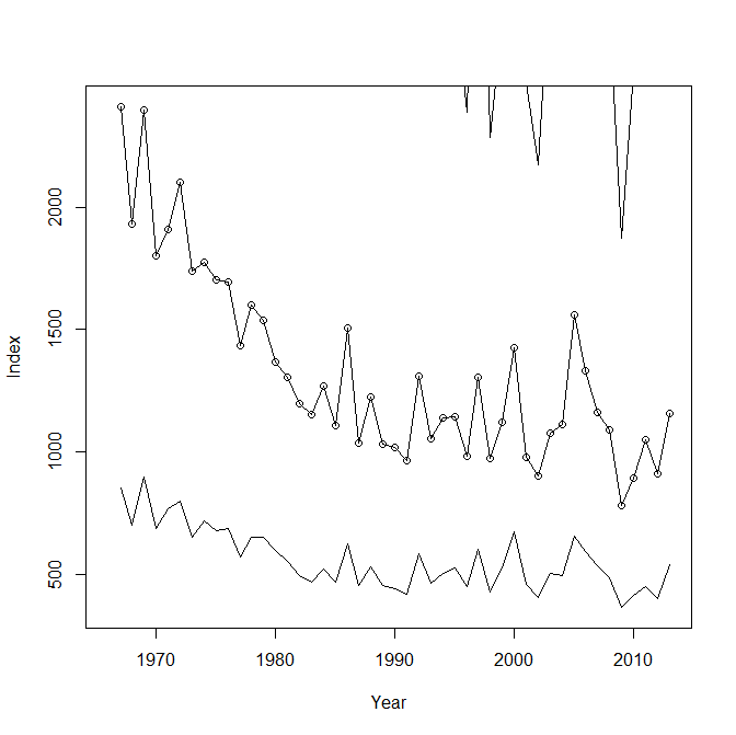
So, how do changes in Franklin’s Gull populations relate to these events? The Breeding Bird Survey provides the best data to understand populations from year-to-year. The 2015 data are a year or more away from being available, but the 1998 invasion may provide some clues here. If 1998 was a great breeding year, we would expect an uptick in records.
The graph below shows data from 1968-2013 in the Prairie Potholes bird conservation region, an area representing an epicenter for Franklin’s Gull during the breeding season. Clearly, there is substantial year-to-year variation. Although there was a significant decline from the late 1960s through the early 1990s, the abundance index appears to plateau since then. However, it is markedly cyclical throughout, with annual peaks and valleys. If 1998 were an exceptional breeding year, and most young survived, we would expect a marked uptick in the abundance in 1999. Instead we see that 1998 is a valley on the graph, with a minor increase in 1999 (and a bigger uptick in 2000). There is obviously more to the picture to understand this, given that overwinter survival, summer weather conditions, habitat change, and a number of other variables are surely at play. In fact, the 1998 invasion itself could have been a high mortality event that depressed winter survival of an otherwise exceptionally productive breeding year. To fully understand this we would need data on breeding productivity (% of birds fledged) from 1998 and other years, which unfortunately is not available. But given what data we do have, breeding productivity does not seem to be an obvious factor here.
Nonetheless, one scenario that may explain the patterns of eastern North American vagrancy in Franklin’s Gulls may well be something like this: gulls have a successful year in terms of their production of young, and then warmer than normal temperatures, and meteorological conditions associated with these temperature anomalies, keep birds in their breeding and migratory staging areas longer. Increased prevalence of strong mid-latitude cyclones associated with these weather conditions then put the birds at greater risk for mass displacement. This at least is a plausible explanation for the 1998 and 2015 invasions. Of course, this is where the excitement of investigating patterns begins – stay tuned for updates as we and our friends at Cape May, Kiptopeke, and the National Weather Service look for evidence supporting these theories and explanations!